Reduction toolbox
Note
This is not intended to be an introduction to image reduction. While performing the steps presented here may be the correct way to reduce data in some cases, it is not correct in all cases.
Logging in ccdproc
All logging in ccdproc is done in the sense of recording the steps performed in image metadata. if you want to do logging in the python sense of the word please see those docs.
There are basically three logging options:
- Implicit logging: No setup or keywords needed, each of the functions below adds a note to the metadata when it is performed.
- Explicit logging: You can specify what information is added to the metadata using the add_keyword argument for any of the functions below.
- No logging: If you prefer no logging be done you can “opt-out” by calling each function with add_keyword=None.
Gain correct and create deviantion image
Uncertainty
An uncertainty can be calculated from your data with create_deviation:
>>> from astropy import units as u
>>> import numpy as np
>>> import ccdproc
>>> img = np.random.normal(loc=10, scale=0.5, size=(100, 232))
>>> data = ccdproc.CCDData(img, unit=u.adu)
>>> data_with_deviatione = ccdproc.create_deviation(data,
...                                              gain=1.5 * u.electron/u.adu,
...                                              readnoise=5 * u.electron)
>>> data_with_deviation.header['exposure'] = 30.0  # for dark subtraction
The uncertainty,  , at pixel
  with value
 is calculated as
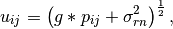
where  is the read noise. Gain is only necessary when the
image units are different than the units of the read noise, and is used only
to calculate the uncertainty. The data itself is not scaled by this function.
is the read noise. Gain is only necessary when the
image units are different than the units of the read noise, and is used only
to calculate the uncertainty. The data itself is not scaled by this function.
As with all of the functions in ccdproc, the input image is not modified.
In the example above the new image data_with_deviation has its uncertainty set.
Gain
To apply a gain to an image, do:
>>> gain_corrected = ccdproc.gain_correct(data_with_deviation, 1.5*u.electron/u.adu)
The result gain_corrected has its data and uncertainty scaled by the gain and its unit updated.
There are several ways to provide the gain, among them as an astropy.units.Quantity, as in the example above, as a ccdproc.Keyword. See to documentation for gain_correct for details.
Clean image
There are two ways to clean an image of cosmic rays. One is to use clipping to create a mask for a stack of images, as described in Image masks/clipping.
The other is to replace, in a single image, each pixel that is several standard deviations from a central value in a region surrounding that pixel. The methods below describe how to do that.
LACosmic
The lacosmic technique identifies cosmic rays by identifying pixels based on a variation of the Laplacian edge detection. The algorithm is an implementation of the code describe in van Dokkum (2001) [1].
Use this technique with cosmicray_lacosmic:
>>> cr_cleaned = ccdproc.cosmicray_lacosmic(gain_corrected, threshold,
...                                         thresh=5, mbox=11, rbox=11,
...                                         gbox=5)
median
Another cosmic ray cleaning algorithm available in ccdproc is cosmicray_median that is analogous to iraf.imred.crutil.crmedian. This technique can be used with ccdproc.cosmicray_median:
>>> cr_cleaned = ccdproc.cosmicray_median(gain_corrected, threshold,
...                                       mbox=11, rbox=11, gbox=5)
Although ccdproc provides functions for identifying outlying pixels and for calculating the deviation of the background you are free to provide your own error image instead.
There is one additional argument, gbox, that specifies the size of the box, centered on a outlying pixel, in which pixel should be grown. The argument rbox specifies the size of the box used to calculate a median value if values for bad pixels should be replaced.
Subtract overscan and trim images
Note
- Images reduced with ccdproc do NOT have to come from FITS files. The discussion below is intended to ease the transition from the indexing conventions used in FITS and IRAF to python indexing.
- No bounds checking is done when trimming arrays, so indexes that are too large are silently set to the upper bound of the array. This is because numpy, which provides the infrastructure for the arrays in ccdproc has this behavior.
Indexing: python and FITS
Overscan subtraction and image trimming are done with two separate functions. Both are straightforward to use once you are familiar with python’s rules for array indexing; both have arguments that allow you to specify the part of the image you want in the FITS standard way. The difference between python and FITS indexing is that python starts indexes at 0, FITS starts at 1, and the order of the indexes is switched (FITS follows the FORTRAN convention for array ordering, python follows the C convention).
The examples below include both python-centric versions and FITS-centric versions to help illustrate the differences between the two.
Consider an image from a FITS file in which NAXIS1=232 and NAXIS2=100, in which the last 32 columns along NAXIS1 are overscan.
In FITS parlance, the overscan is described by the region [201:232, 1:100].
If that image has been read into a python array img by astropy.io.fits then the overscan is img[0:100, 200:232] (or, more compactly img[:, 200:]), the starting value of the first index implicitly being zero, and the ending value for both indices implicitly the last index).
One aspect of python indexing may particularly surprising to newcomers: indexing goes up to but not including the end value. In img[0:100, 200:232] the end value of the first index is 99 and the second index is 231, both what you would expect given that python indexing starts at zero, not one.
Those transitioning from IRAF to ccdproc do not need to worry about this too much because the functions for overscan subtraction and image trimming both allow you to use the familiar BIASSEC and TRIMSEC conventions for specifying the overscan and region to be retained in a trim.
Overscan subtraction
To subtract the overscan in our image from a FITS file in which NAXIS1=232 and NAXIS2=100, in which the last 32 columns along NAXIS1 are overscan, use subtract_overscan:
>>> # python-style indexing first
>>> oscan_subtracted = ccdproc.subtract_overscan(cr_cleaned,
...                                              overscan=cr_cleaned[:, 200:],
...                                              overscan_axis=1)
>>> # FITS/IRAF-style indexing to accomplish the same thing
>>> oscan_subtracted = ccdproc.subtract_overscan(cr_cleaned,
...                                              fits_section='[201:232,1:100]',
...                                              overscan_axis=1)
Note well that the argument overscan_axis always follows the python convention for axis ordering. Since the order of the indexes in the fits_section get switched in the (internal) conversion to a python index, the overscan axis ends up being the second axis, which is numbered 1 in python zero-based numbering.
With the arguments in this example the overscan is averaged over the overscan columns (i.e. 2000 through 2031) and then subtracted row-by-row from the image. The median argument can be used to median combine instead.
This example is not very realistic: typically one wants to fit a low-order polynomial to the overscan region and subtract that fit:
>>> from astropy.modeling import models
>>> poly_model = models.Polynomial1D(1)  # one-term, i.e. constant
>>> oscan_subtracted = ccdproc.subtract_overscan(cr_cleaned,
...                                              overscan=cr_cleaned[:, 200:],
...                                              overscan_axis=1,
...                                              model=poly_model)
See the documentation for astropy.modeling.polynomial for more examples of the available models and for a description of creating your own model.
Trim an image
The overscan-subtracted image constructed above still contains the overscan portion. We are assuming came from a FITS file in which NAXIS1=2032 and NAXIS2=1000, in which the last 32 columns along NAXIS1 are overscan.
Trim it using trim_image,shown below in both python- style and FITS-style indexing:
>>> # FITS-style:
>>> trimmed = ccdproc.trim_image(oscan_subtracted,
...                              fits_section='[1:200, 1:100]')
>>> # python-style:
>>> trimmed = ccdproc.trim_image(oscan_subtracted[:, :200])
Note again that in python the order of indices is opposite that assumed in FITS format, that the last value in an index means “up to, but not including”, and that a missing value implies either first or last value.
Those familiar with python may wonder what the point of trim_image is; it looks like simply indexing oscan_subtracted would accomplish the same thing. The only additional thing trim_image does is to make a copy of the image before trimming it.
Note
By default, python automatically reduces array indices that extend beyond the actual length of the array to the actual length. In practice, this means you can supply an invalid shape for, e.g. trimming, and an error will not be raised. To make this concrete, ccdproc.trim_image(oscan_subtracted[:, :200000000]) will be treated as if you had put in the correct upper bound, 200.
Subtract bias and dark
Both of the functions below propagate the uncertainties in the science and calibration images if either or both is defined.
Assume in this section that you have created a master bias image called master_bias and a master dark image called master_dark that has been bias-subtracted so that it can be scaled by exposure time if necessary.
Subtract the bias with subtract_bias:
>>> fake_bias_data = np.random.normal(size=trimmed.shape)  # just for illustration
>>> master_bias = ccdproc.CCDData(fake_bias_data,
...                               unit=u.electron,
...                               mask=np.zeros(trimmed.shape))
>>> bias_subtracted = ccdproc.subtract_bias(trimmed, master_bias)
There are several ways you can specify the exposure times of the dark and science images; see subtract_dark for a full description.
In the example below we assume there is a keyword exposure in the metadata of the trimmed image and the master dark and that the units of the exposure are seconds (note that you can instead explicitly provide these times).
To perform the dark subtraction use subtract_dark:
>>> master_dark = master_bias.multiply(0.1)  # just for illustration
>>> master_dark.header['exposure'] = 15.0
>>> dark_subtracted = ccdproc.subtract_dark(bias_subtracted, master_dark,
...                                         exposure_time='exposure',
...                                         exposure_unit=u.second,
...                                         scale=True)
Note that scaling of the dark is not done by default; use scale=True to scale.
Correct flat
Given a flat frame called master_flat, use flat_correct to perform this calibration:
>>> fake_flat_data = np.random.normal(loc=1.0, scale=0.05, size=trimmed.shape)
>>> master_flat = ccdproc.CCDData(fake_flat_data, unit=u.electron)
>>> reduced_image = ccdproc.flat_correct(dark_subtracted, master_flat)
As with the additive calibrations, uncertainty is propagated in the division.
The flat is scaled by the mean of master_flat before dividing.
If desired, you can specify a minimum value the flat can have (e.g. to prevent division by zero). Any pixels in the flat whose value is less than min_value are replaced with min_value):
>>> reduced_image = ccdproc.flat_correct(dark_subtracted, master_flat,
...                                      min_value=0.9)
| [1] | van Dokkum, P; 2001, “Cosmic-Ray Rejection by Laplacian Edge Detection”. The Publications of the Astronomical Society of the Pacific, Volume 113, Issue 789, pp. 1420-1427. doi: 10.1086/323894 |